2 Methodology
2.1 Data Collection
The data set for this research is from **RSV Hospitalization Surveillance Network (RSV-NET)** (one of CDC research and surveillance platforms) ,which conducts population-based surveillance system for laboratory-confirmed COVID-19, RSV, and influenza-associated hospitalizations in the US among children younger than 18 years of age and adults.[8]
RSV-NET has been collecting RSV-associated hospitalizations in adults and children since 2018-2019 season from 58 counties in 12 states, including California, Colorado, Connecticut, Georgia, Maryland, Michigan, Minnesota, New Mexico, New York, Oregon, Tennessee, and Utah. Almost 9% of the U.S. population is covered and reported by the RSV-NET.
2.2 About this Dataset
Time frame: In season 2018-2019, 2019-2020, data collected is from October 1 to April 30. In season 2020-2021, 2021-2022, 2022-2023, data collected is from October 1 to October 1 next year.
How an entry is made in data set:
A case is defined by laboratory-confirmed RSV in a person who Lives in a defined RSV-NET surveillance area AND Tests positive for RSV within 14 days before or during hospitalization. Evidence of RSV infection can be obtained through several laboratory tests.
Variables:
In the original data set, it has 8 columns which are described in below table
Column Name Description State Represents the state name from which data was collected. Entire state means all 9 states considered in this dataset. MMWR Year Represents Year MMWR Week Represents week of that year. MMWR - Morbidity and Mortality Weekly Report, is prepared by the Centers for Disease Control and Prevention (CDC). Season As the data is collected between October to April, this represents the duration of the year. Age Category Age limit Sex Male/Female Race Black, White, American Indian/Alaska Native and Asian/Pacific Islander people are categorized as non-Hispanic. Hispanic people could be of any race. If Hispanic ethnicity was unknown, non-Hispanic ethnicity was assumed. Rate calculated as the number of residents in a surveillance area who are hospitalized with laboratory-confirmed RSV divided by the total population estimate for that area. [NCHS bridged-race population](https://www.cdc.gov/nchs/nvss/bridged_race.htm) estimates are used as denominators for rate calculations. The data was last updated on 17th November 2022. We have considered two sets of data, one with last 12 months of YTD data and another one with 24 months of YTD data for our calculations.
2.3 Methods
2.3.1 Why Polynomial Regression?
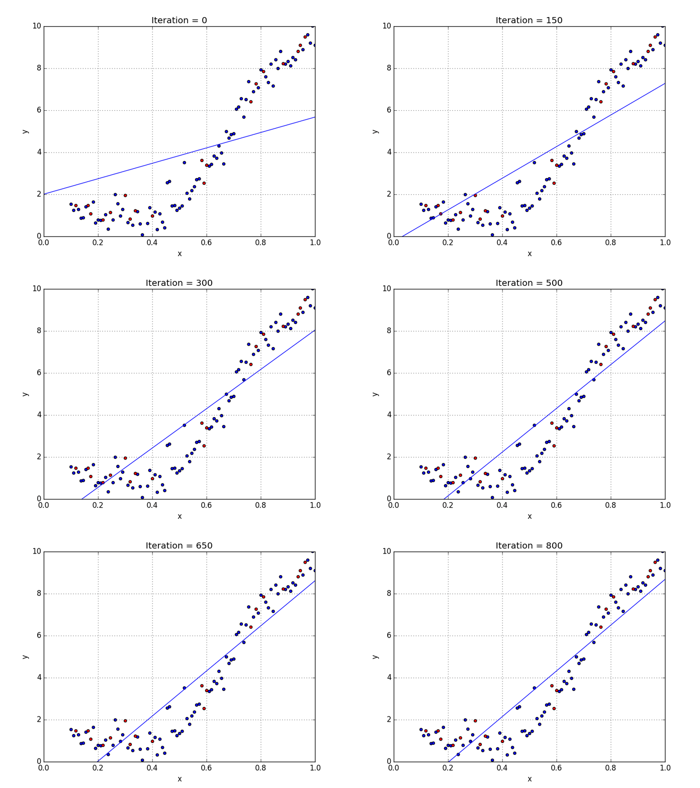
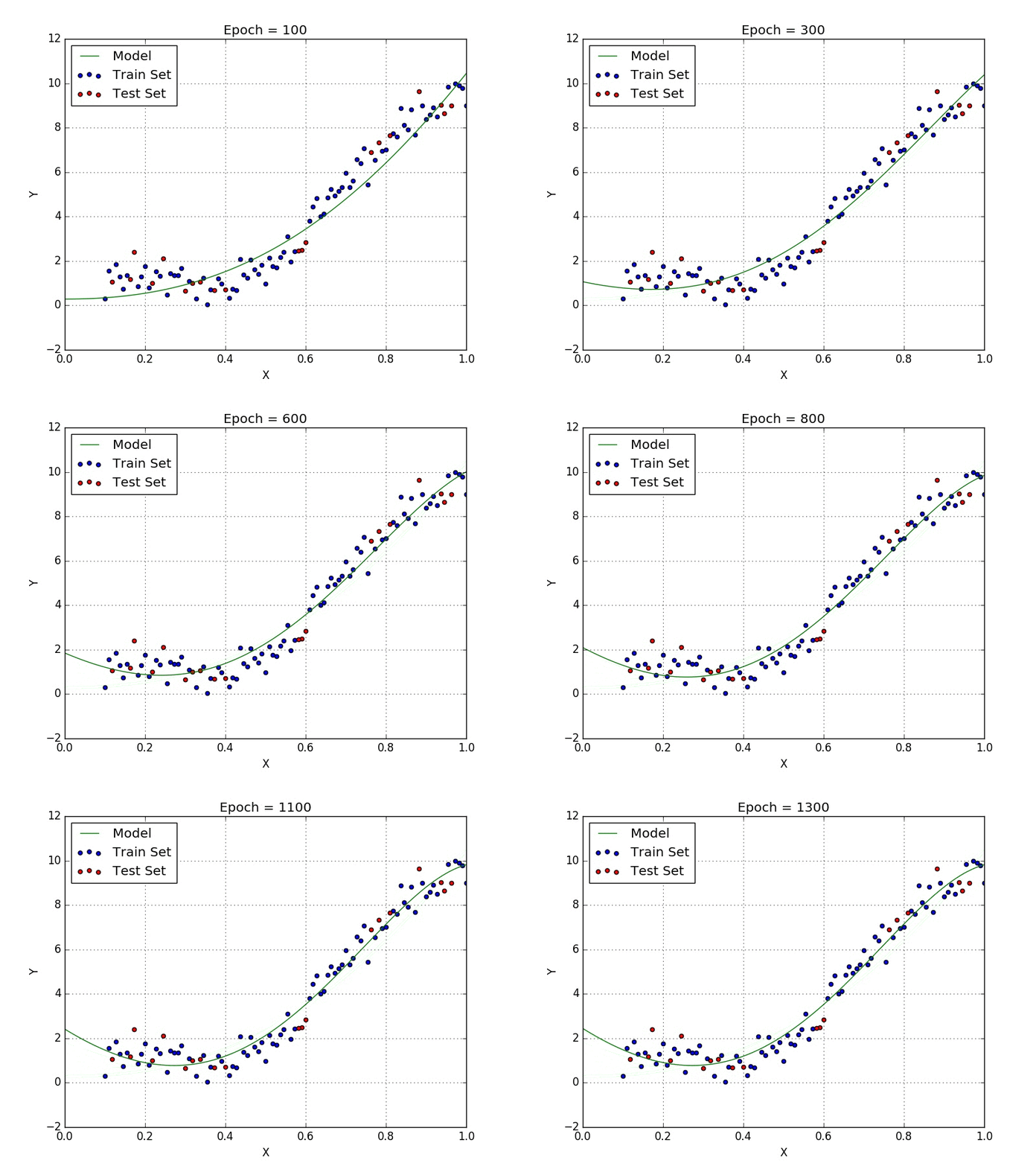
In simple linear regression algorithm only works when the relationship between the data is linear, suppose if we have non-linear data then linear regression will not be capable to draw a best-fit line and it fails in such conditions. Consider the below diagram which has a non-linear relationship and you can see the Linear regression results on it, which does not perform well and doesn’t come close to reality. Hence, we introduce polynomial regression to overcome this problem, which helps identify the curvilinear relationship between independent and dependent variables.

2.3.2 How Polynomial Regression Overcomes the problem of Non-Linear data?

Polynomial regression is a form of Linear regression where only due to the Non-linear relationship between dependent and independent variables we add some polynomial terms to linear regression to convert it into Polynomial regression.
Suppose we have X as Independent data and Y as dependent data. Before feeding data to a mode in preprocessing stage we convert the input variables into polynomial terms using some degree.
Consider an example my input value is 35 and the degree of a polynomial is 2 so I will find 35 power 0, 35 power 1, and 35 power 2 And this helps to interpret the non-linear relationship in data.
The equation of polynomial becomes something like this.[9]
y = 𝛽0 + 𝛽1x1 + 𝛽2x12 + … + 𝛽nx1n
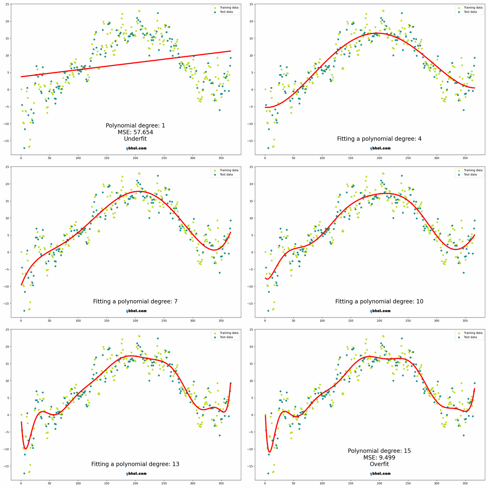
The degree of order which to use is a Hyper-parameter, and we need to choose it wisely. But using a high degree of polynomial tries to over-fit the data and for smaller values of degree, the model tries to under-fit so we need to find the optimum value of a degree.
If you see the equation of polynomial regression carefully, then we can see that we are trying to estimate the relationship between coefficients and y. And the values of x and y are already given to us, only we need to determine coefficients and the degree of coefficient here is 1 only, and degree one represents simple linear regression Hence, Polynomial regression is also known as polynomial Linear regression.

In statistics, polynomial regression is a form of regression analysis in which the relationship between the independent variable x and the dependent variable y is modelled as an nth degree polynomial in x. Polynomial regression fits a nonlinear relationship between the value of x and the corresponding conditional mean of y, denoted E(y |x). Although polynomial regression fits a nonlinear model to the data, as a statistical estimation problem it is linear, in the sense that the regression function E(y | x) is linear in the unknown parameters that are estimated from the data. For this reason, polynomial regression is considered to be a special case of multiple linear regression. The explanatory (independent) variables resulting from the polynomial expansion of the “baseline” variables are known as higher-degree terms. Such variables are also used in classification settings[10].